Why Prefill and Decode Should Not Share a GPU
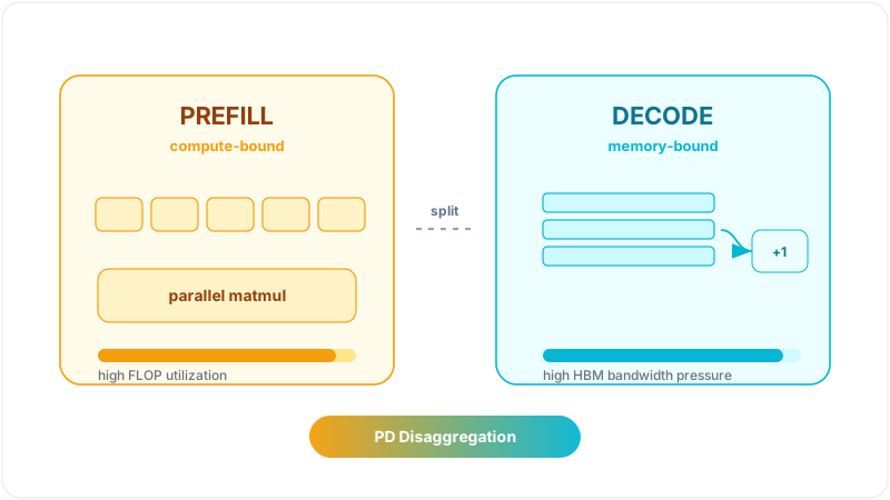
A single LLM request looks like one operation from the API boundary, but inside the GPU it is really two workloads with opposite personalities.
Prefill reads the whole prompt, processes all input tokens in parallel, builds the initial KV cache, and produces the first output token. It wants large matrix multiplications, large enough batches, and high FLOP utilization. Decode emits one token at a time. Each step computes very little, but it repeatedly reads the growing KV cache from HBM. It wants stable memory bandwidth, predictable scheduling, and no surprise long prompt blocking the next token.
Putting both phases on the same GPU is convenient, but it turns serving into a permanent compromise. Prefill is compute-bound. Decode is memory-bound. Prefill wants bigger batches. Decode wants short, regular per-token steps. Prefill-Decode disaggregation, or PD disaggregation, starts from a blunt systems observation: if first-token work and next-token work stress different physical resources, deploy them on different GPU pools and tune them independently.
Prefill and Decode Are Two Different Workloads
The easiest way to understand PD disaggregation is to stop saying “one inference request” too early. The request has at least two phases.
During prefill, the full prompt is already known. Attention over the prompt can be computed in parallel, so the GPU sees dense matrix work. Long prompts can take hundreds of milliseconds, but the expensive part is mostly math: large GEMMs, high tensor-core utilization, and a natural preference for batching.
During decode, generation becomes autoregressive. At step , the model can only produce the next token. To compute attention for that one new token, it has to read keys and values for the previous tokens. The arithmetic per step is small; the memory traffic is not. Tensor cores can sit idle while the kernel waits on HBM bandwidth.
| Phase | What it does | Physical bottleneck | User-facing metric |
|---|---|---|---|
| Prefill | Processes the prompt in parallel and creates KV cache | FLOPs / compute | TTFT, or time to first token |
| Decode | Reads KV cache repeatedly and emits one token per step | HBM bandwidth | TPOT / ITL, or per-token latency |
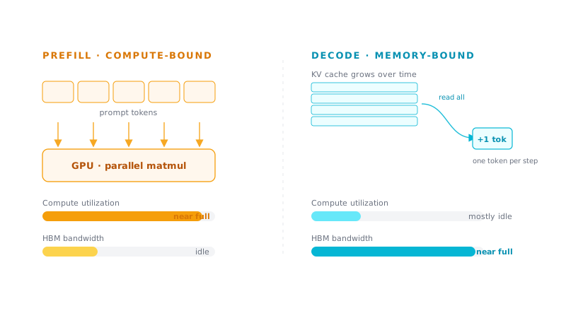
Figure 1. The two faces of one inference request: prefill fills compute, while decode fills memory bandwidth.
The analogy I use is a warehouse. Prefill is loading a truck once: it is heavy, but the work is concentrated. Decode is sending a runner back to the warehouse for one item at a time, except the runner has to scan the whole growing history on every trip. One phase is limited by lifting power; the other is limited by repeated movement.
This difference is not a terminology detail. It explains why the same batching policy, placement policy, and GPU allocation policy cannot be simultaneously ideal for both phases.
KV Cache Is the Physical Root
Decode is memory-bound because of KV cache. For every processed token, every transformer layer stores key and value vectors. A useful first-order formula is:
Here, is for key and value, is the number of layers, is the number of KV heads, is the head dimension, is sequence length, and is batch size. For a fixed model and dtype, the KV cost per token is almost a constant, so total KV memory grows linearly with context length.
This is why MQA, GQA, and MLA are not minor implementation tricks for serving. They attack the same formula:
- MQA shares one KV head across all query heads.
- GQA shares KV heads across query groups and reduces
num_kv_heads. - MLA, used by DeepSeek-style models, stores a compressed latent representation instead of a full per-head K/V cache and reconstructs what attention needs later.
Take Qwen2.5-32B in BF16 as a concrete example. It has 64 layers, 40 query heads, 8 KV heads through GQA, and head_dim = 128. The KV cache per token is:
That means one request at 8K context uses about 2 GB of KV cache. At 32K context, it uses about 8 GB. If the same model used ordinary MHA with 40 KV heads, the per-token KV would be 5x larger, roughly 1.25 MB per token, and 8K context would require about 10 GB for one request.
The calculation is just the formula translated into code:
def kv_cache_bytes(
    num_layers: int,
    num_kv_heads: int,
    head_dim: int,
    seq_len: int,
    batch_size: int,
    dtype_bytes: int = 2,
) -> int:
    # 2 = Key + Value; the remaining terms correspond to model and workload dimensions.
    return 2 * num_layers * num_kv_heads * head_dim * seq_len * batch_size * dtype_bytes


# Qwen2.5-32B with GQA: 64 layers, 8 KV heads, head_dim 128, BF16.
per_token = kv_cache_bytes(64, 8, 128, seq_len=1, batch_size=1)
print(per_token / 1024)                                  # 256.0 KB per token
print(kv_cache_bytes(64, 8, 128, 8192, 1) / 1024**3)     # 2.0 GB at 8K context
print(kv_cache_bytes(64, 8, 128, 32768, 1) / 1024**3)    # 8.0 GB at 32K context
Now connect that number to decode. Every decode step appends the new token’s K/V, then computes attention between the new query and all historical K/V. Schematic code makes the memory pattern obvious:
class KVCacheAttention(nn.Module):
    def forward(self, x, kv_cache=None):
        q, k, v = self.qkv_proj(x).chunk(3, dim=-1)

        if kv_cache is not None:
            # Decode: append the new token's K/V to the growing history.
            k = torch.cat([kv_cache.k, k], dim=1)
            v = torch.cat([kv_cache.v, v], dim=1)

        kv_cache.update(k, v)

        # One new query attends over all historical K/V.
        attn = (q @ k.transpose(-2, -1)) * self.scale
        out = attn.softmax(dim=-1) @ v
        return out, kv_cache
The important line is not the concatenation itself; it is the fact that k and v grow with the generated history and are read again on every step. Context gets longer, the memory region gets larger, and decode slows down because it must keep moving bytes.
In roofline terms, decode often has very low arithmetic intensity. A rough matrix-vector view gives something around 1 FLOP/byte, far below the H100 ridge point of roughly 295 FLOP/byte, based on 989 TFLOPS divided by 3.35 TB/s. Decode sits far down the bandwidth slope. Prefill, with larger matrix-matrix work over the prompt, sits much closer to the compute roof.
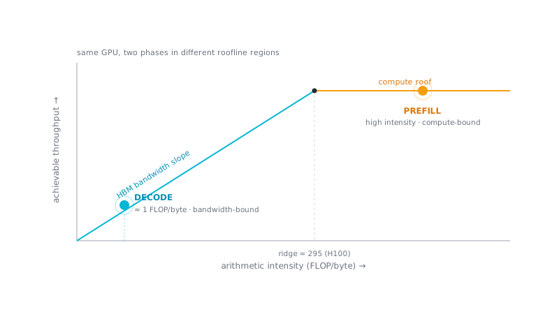
Figure 2. In a roofline view, decode lands on the bandwidth slope because every step rereads KV cache, while prefill is closer to the compute roof.
KV cache therefore plays two roles in PD disaggregation. It is the reason decode is memory-bound, and it is the object that must move from the prefill pool to the decode pool. Smaller KV cache helps twice: it reduces decode bandwidth pressure and it reduces transfer cost between P and D.
Mixed Scheduling Makes the Phases Hurt Each Other
Modern inference engines commonly use continuous batching. Instead of waiting for a static batch to finish, they keep admitting new requests and advancing existing decode requests step by step. This is the right general direction for utilization, but it also mixes prefill and decode on the same GPU.
The classic failure mode is prefill blocking decode. A new request with a long prompt enters the batch. Its prefill phase wants to occupy the GPU with dense compute for hundreds of milliseconds. Existing requests that were already streaming tokens now wait for their next decode step. The user does not see “a scheduling conflict”; the user sees smooth output suddenly pause. That pause is an ITL or TPOT spike.

Figure 3. A long prefill job can interrupt an otherwise stable decode stream, causing a visible inter-token latency spike.
The reverse trade-off exists too. If the scheduler protects decode too aggressively, it limits prefill batch size and leaves prefill throughput on the table. The two phases want different scheduling shapes:
- Prefill wants larger chunks and larger batches to maximize compute efficiency.
- Decode wants short, predictable scheduling intervals to minimize per-token latency spikes.
- A single shared GPU forces the scheduler to trade one SLO against the other.
Chunked prefill is the best-known non-disaggregated mitigation. It splits a long prefill into smaller pieces and interleaves those chunks with decode steps. This is practical and often excellent on a single node or a moderate-scale deployment. But it is still an intra-GPU scheduling technique. Prefill and decode continue to share the same hardware resources.
PD disaggregation is more aggressive. It says the problem is not only that the phases need better time slicing. The phases want different resource pools.
What PD Disaggregation Changes
In a PD-disaggregated system, a request first goes to a prefill worker or prefill GPU group. The prefill side processes the prompt, creates the KV cache, and emits the first token. Then the KV cache is transferred over a high-speed interconnect, such as NVLink, RDMA, or InfiniBand, to a decode worker. The decode side receives that KV cache, continues autoregressive generation, and streams tokens back to the client.
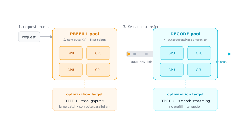
Figure 4. PD disaggregation computes KV cache in the prefill pool, transfers it over fast interconnect, and continues generation in the decode pool.
The benefit is SLO decoupling. Prefill nodes can be optimized for TTFT and throughput. They can use larger prefill batches, prompt-heavy scheduling, and compute-oriented parallelism. Decode nodes can be optimized for TPOT and streaming smoothness. They are not interrupted by a surprise long prompt.
The cost is the KV transfer. A prompt’s KV cache can be hundreds of MB or multiple GB, depending on context length, model size, dtype, and KV compression. If the interconnect is slow, the transfer latency can erase the benefit of disaggregation. This is why PD disaggregation is most compelling in large serving clusters with fast interconnects, latency-sensitive workloads, and enough traffic to keep both pools busy.
The clean mental model is: pay one KV movement cost to stop forcing two opposite workloads to fight over the same GPU schedule.
vLLM and SGLang: Same Skeleton, Different Contract
The public implementations in vLLM and SGLang share the same high-level skeleton: separate prefill and decode instances, a proxy or router that pairs them, and a KV transfer path backed by RDMA-capable systems. The difference is how each project abstracts the transfer and handshake.
vLLM: Connector First
vLLM frames disaggregation around a pluggable KVConnector abstraction. Instead of hard-coding one transport path into the engine, vLLM lets the system use different backends for KV movement. Publicly discussed paths include NIXL, Mooncake, LMCache, and P2P NCCL for native xPyD-style deployments.
The common flow is:
- A proxy selects a prefill instance and a decode instance, often as a 1P1D pair.
- The prompt is sent to the prefill side, sometimes with
max_tokensadjusted so the prefill side only needs to produce the first token. - The prefill worker computes KV cache.
- The prefill side pushes KV to the decode side through the configured connector.
- Decode resumes generation and streams the rest of the response.
This design makes vLLM feel like an engine plus a connector ecosystem. The upside is backend optionality and integration with a fast-moving serving engine. The caveat is maturity and deployment complexity. Public docs still treat parts of PD/xPyD as experimental. Some deployments also rely on external orchestration, such as llm-d or Dynamo-style systems. It is best understood as a tool for shaping TTFT and ITL, not as a magic switch that automatically increases throughput.
SGLang: Built-in Components and a Fixed Handshake
SGLang exposes a more built-in PD topology: proxy, prefill server, decode server, and sglang_router for routing, load balancing, and fault handling. The transfer engine is usually Mooncake or NIXL, with RDMA and non-blocking transfer as the important systems primitives.
The subtle but important difference is the order of the handshake. In SGLang’s PD path, the decode side first prepares the destination memory for the incoming KV cache. Only then does it signal the prefill side to compute and write KV into the reserved decode memory. It is not “prefill computes and then finds somewhere to put KV”; it is “decode reserves the slot, then tells prefill to fill it.”
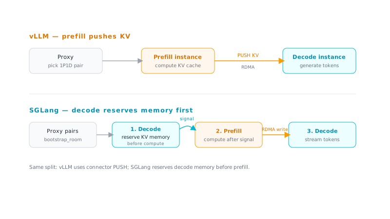
Figure 5. vLLM and SGLang share the same P/D split, but differ in the KV transfer contract and handshake order.
SGLang also exposes several engineering features that matter in real deployments: dynamic connections, non-blocking KV transfer, heterogeneous P/D tensor parallelism, and RDMA transfer. Heterogeneous TP is useful because prefill and decode may want different parallel configurations. The caveat is that non-MLA models can require staging buffers when the P and D layouts do not match cleanly.
The short comparison is:
| Dimension | vLLM | SGLang |
|---|---|---|
| Abstraction | Pluggable KVConnector ecosystem | Built-in proxy, prefill, decode, router |
| Typical transfer backends | NIXL, Mooncake, LMCache, P2P NCCL | Mooncake, NIXL |
| Control flow | Prefill computes, then pushes KV | Decode reserves memory, then triggers prefill |
| Strength | Backend optionality and engine integration | Explicit PD serving topology and handshake |
| Caveat | Some PD paths remain experimental | More opinionated stack and protocol |
Mooncake is worth calling out because it represents a broader KV-cache-centric direction. It is not merely a point-to-point transfer helper. Mooncake-style systems pool CPU, DRAM, SSD, and RDMA resources into a global KV cache layer. A central scheduler can place requests based on KV distribution and load, reuse prefix KV across requests, and compute only missed deltas. This is the same serving family as DistServe and Splitwise: the system is organized around the fact that KV cache is the central object in long-context serving.
The Cost Side: Transfer and P:D Scheduling
Disaggregation is not free. It converts “two workloads competing on one GPU” into a distributed systems problem. Whether it is worth doing depends on two costs.
The first cost is cross-node KV transfer. A request’s KV cache can be hundreds of MB or multiple GB, growing linearly with prompt length, layer count, KV head count, batch size, and dtype. If the network cannot move that KV quickly enough, the transfer latency can eat the benefit that disaggregation was supposed to create. This is why production PD work spends so much energy on hierarchical transfer, overlap between transfer and useful work, selective or on-demand movement, and careful placement.
The second cost is the P:D ratio. How many GPUs should be prefill GPUs, and how many should be decode GPUs? The answer depends on the traffic shape.
| Workload shape | Typical scenario | Allocation pressure |
|---|---|---|
| Long input, short output | RAG, document QA, long-context summarization | More prefill capacity |
| Short input, long output | Agentic reasoning, long-form generation | More decode capacity |
| Mixed online traffic | Real production traffic | Dynamic P:D adjustment |
If the ratio is wrong, one side queues while the other side idles. A good PD system therefore needs more than fast transport. It also needs routing, admission control, placement, and autoscaling logic that understand the separate bottlenecks of P and D.
The practical decision rule is simple: PD disaggregation is attractive for large online serving, strict latency SLOs, long-context or mixed workloads, and clusters with fast interconnects. For small single-node deployments, weak interconnects, or low traffic, continuous batching plus chunked prefill is often the better engineering trade.
Two Easy Confusions
PD disaggregation is an inference-time optimization. It is not the same thing as “training-inference disaggregation” in RL post-training systems.
In RLHF, PPO, GRPO, DAPO, and agentic RL systems, people also split rollout from training. That is a higher-level architecture: one cluster samples responses, another cluster updates model weights, and the system manages policy lag, replay buffers, partial rollout, and off-policy correction. PD disaggregation can live inside the rollout service because rollout is inference. But it is not the same split. The former happens inside one generation request; the latter happens between sampling and parameter updates.
There is also no PD disaggregation in ordinary teacher-forced training. SFT and pretraining know the target sequence in advance, so the forward pass computes all positions in parallel. That looks much more like prefill than decode. The step-by-step decode phase exists only when the model is autoregressively generating unknown future tokens. PD can appear in an RL training pipeline only indirectly, through the rollout stage.
Summary
PD disaggregation works because it follows the physical shape of LLM inference: prefill is compute-bound, decode is memory-bound, and KV cache is both the reason they differ and the object that must cross the boundary.
| Decision point | Keep mixed scheduling | Use PD disaggregation |
|---|---|---|
| Deployment size | Single node or small cluster | Large serving cluster |
| Interconnect | Ordinary or limited bandwidth | RDMA, NVLink, InfiniBand class |
| Main mitigation | Continuous batching, chunked prefill | Separate P/D pools and KV transfer |
| Best workload | Moderate context, relaxed latency | Long context, mixed traffic, tight ITL |
| Main risk | Prefill and decode interfere | KV transfer and P:D scheduling complexity |
The key is not that PD disaggregation is always better. It is better when the cost of moving KV cache is lower than the cost of forcing two opposite workloads to share the same GPU schedule. From continuous batching to chunked prefill to full PD disaggregation, the serving stack keeps moving in the same direction: admit that prefill and decode want different things, then separate them as much as the deployment can afford.
PD disaggregation is the moment an inference system stops pretending that first-token work and next-token work are the same workload.